Reference Manual (RM #47) Chapter 3: Characterizing the Acoustic Environment

RM-47 Home

DRAFT: Preliminary internal document in review/ Do not cite

This is an internal website intended to capture current approaches and knowledge base from the Natural Sounds & Night Skies Division in order to provide guidance to the field in an easy, user friendly format. It is still under development and this version was made available solely for this internal review. Following review, and prior to formal internal agency vetting, pages will be inactivated in order to incorporate input.

3. Characterizing the Acoustic Environment

A critical step in the process of preserving, protecting, and restoring acoustic resources in parks is characterizing the acoustic environment. In many cases, this is achieved through detailed analysis of data collected in parks over 30 days or more. Once natural ambient sound levels have been calculated, the difference between natural and existing levels can be assessed. By comparing these differences throughout the day, or among different sites, park managers gain insight into how the acoustical environment is affected by human activity. Click here to see a list of acoustic measurement summary reports produced by NPS.

Characterizing the acoustic environment in both terrestrial and aquatic habitats may also include identifying the presence of vocalizing species or levels of bio-acoustic activity. Animals produce sounds for a variety of biological functions such as defending territories, attracting mates, deterring predators, navigation, finding food, and maintaining contact in a social group. Characterizing these acoustic behaviors can provide valuable insights into the spatial and temporal scales over which individuals and populations interact as well as the timing of ecological processes. For example, acoustic recordings paired with analysis of bio-acoustic activity revealed shifts in songbird phenology in Glacier Bay National Park (Buxton et al. 2016). Everglades National Park has paired underwater acoustic recording devices with measures of the oceanographic conditions (e.g. salinity) of Florida Bay to determine if bio-acoustic activity can provide an indicator of changes in the ecosystem.

Understanding temporal trends in sound levels provides a gauge for the changes induced by anthropogenic and climate stressors on the acoustic environment. In addition, long-term acoustic monitoring can inform effectiveness of management decisions or identify possible mitigation efforts. For example, Denali National Park has been collecting acoustic recordings throughout the park since 2001 to understand conditions of the acoustic environment. In 2014, NPS became part of an inter-agency partnership with the National Oceanic and Atmospheric Administration (NOAA) to understand long-term trends in ocean noise, so acoustic monitoring equipment was deployed in National Park of American Samoa and Buck Island Reef National Monument.

Figure 1. Daily spectrogram (from 00:00:00 time to 23:59:59) with sound level plotted as a function of time (x-axis) and frequency (y-axis). The color scale reveals how loud a sound is: blue and purple portions of the plot are quiet, while yellow and white events are loud.

3.1 Visual Analysis of Acoustic Data

The collection of several weeks of continuous audio and sound pressure levels has been made easier by new instruments, but 73 million data points and 600 hours of audio is an overwhelming listening exercise. The current protocol is to subsample the data set, and listen to a few hours of the several hundred in order to document broad trends in audibility of noise sources.

A useful method for presenting and reviewing long-term acoustic datasets is the daily spectrogram (Figure 1), a type of plot showing sound level as a function of time and frequency. Traditionally, spectrograms were used to show fine detail over short time spans. NSNSD developed an innovative approach, using this method to visualize acoustic data over longer timescales, such as a full day. Daily spectrograms do not show the nuances of single events, such as individual birdcalls; however, general patterns, like the dawn chorus, are still visible. Aircraft, vehicles, voices, animal calls, thunder, and other sources are all discernible. In this daily spectrogram figure, there are six distinct high altitude aircraft events (which appear as bright yellow markings), beginning in the 16:00 hour, and ending in the 18:00 hour. Bird song is represented by small, dotted lines concentrated in the morning hours above 4000 Hz.

Figure 2. Screenshot from Sound Pressure Level Annotation Tool (SPLAT). This program allows the user to display one hour of detailed acoustic data, manually identify events, extract sound level information for selected events, and extract audio clips for sharing.

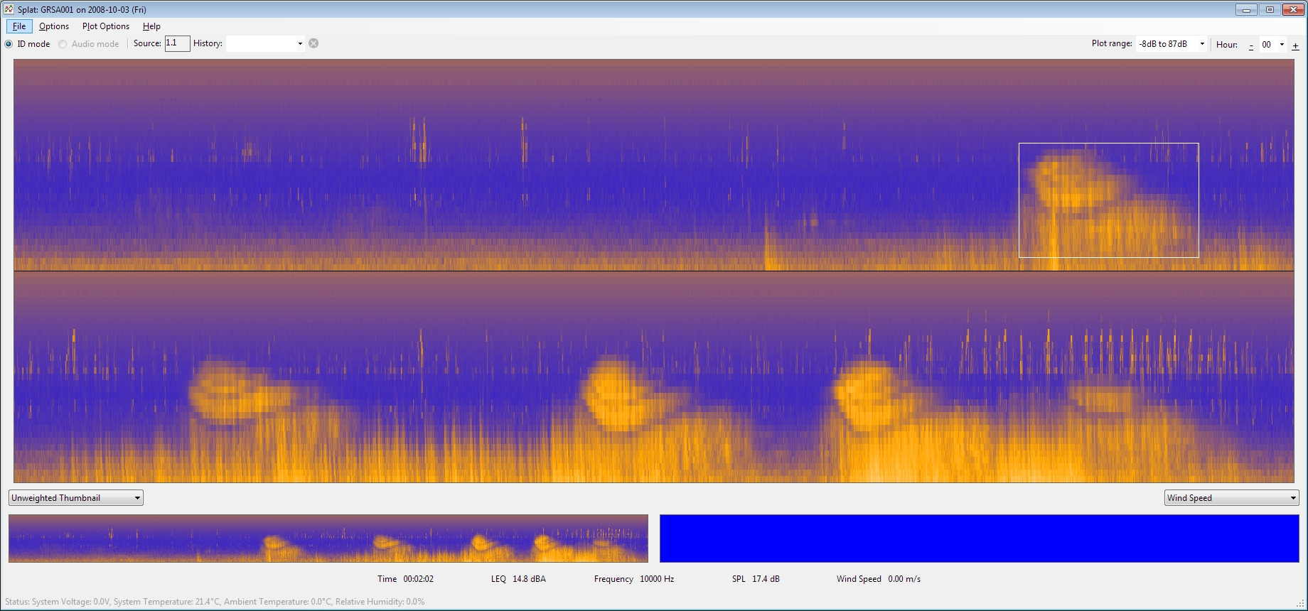
The Natural Sounds and Night Skies Division (NSNSD) has developed a visual analysis tool to log noise events and automatically calculate metrics based on event frequency. The continuous audio is linked to the program, so if the user finds an unknown event, they can highlight it and listen to the corresponding audio. A screenshot from Sound Pressure Level Annotation Tool (SPLAT) is provided in Figure 2. For step-by-step instructions for analyzing acoustic data with SPLAT, see the Acoustic Monitoring Training Manual [PDF]. Annotating a portion of the acoustic data with SPLAT produces a detailed inventory of the types of sounds audible at the site, when they are audible (by hour), and how often they are audible.

Figure 3: Screenshot of Listening Center, a program designed to facilitate analysis of acoustic data by playing a subsample of audio data. Three sound clips are displayed at the top of the window.

3.2 Auditory Analysis of Acoustic Data

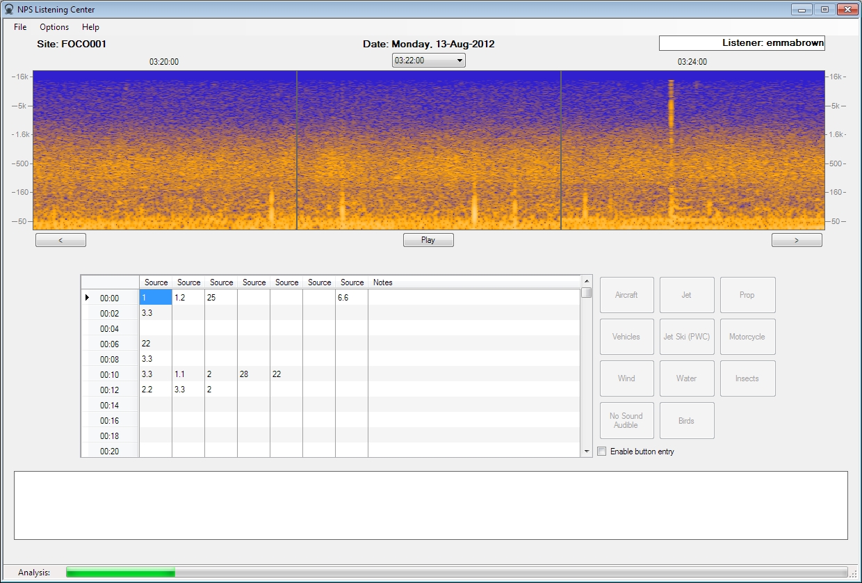
In datasets where visual analysis is difficult (for instance, where many sound events frequently overlap), an auditory analysis tool has also been developed. The Listening Center program (Figure 3) plays short audio clips that have been subsampled from a full day of audio recordings. After each clip is played, the user enters which sounds were audible into an integrated spreadsheet. Annotating a portion of the acoustic data with Listening Center produces a detailed inventory of the types of sounds audible at the site, when they are audible (by hour), and how often they are audible.

For step-by-step instructions for analyzing acoustic data with Listening Center, see the Acoustic Monitoring Training Manual [PDF]. Many National Park Service datasets are analyzed at Colorado State University Listening Lab through a cooperative agreement under the Cooperative Ecosystems Studies Unit (CESU) network.

3.3 Estimating Natural Ambient Levels

It is important for parks to determine background sound levels because these represent the minimum level of acoustical signals that can be detected, identified, and localized. The natural ambient (L_nat) provides an estimate of what the ambient sound level at a site would be if all anthropogenic sources were removed. L_nat is also the baseline condition and the standard against which current acoustical conditions and potential impacts will be measured (NPS Management Policies 8.2.3). The process of identifying anthropogenic noise events (see section 3.1 or 3.2) enables us to calculate natural ambient sound levels. Because sound levels vary substantially throughout the day, natural ambient is calculated on an hourly basis. Natural ambient (L_nat) is calculated using the following approach (an example follows the bullets):

• Review each hour of data.
• Calculate the percentage of time that noise is audible (P_H).
• Remove the percentage of audible noise (P_H) from the loudest measurements in the hourly data.
• Calculate the median of the remaining data to produce the natural ambient (L_nat).
• Lnat is defined by equation (1). For a given hour (or other specified time period), L_natis calculated to be the decibel level exceeded x percent of the time.

Example: After thorough analysis a user discovers that noise is audible at a national park site for 40% of an hour. Therefore, for this hour, P_H = 40. To calculate the natural ambient sound level, use equation (1).

The L_nat is equal to the L₇₀, or the sound level exceeded 70% of the time during the hour. If one were to repeat this process for all 24 hours, a plot such as Figure 4 could be produced.

• 

  How to calculate natural ambient

  Video showing how natural ambient is calculated for an hour

  Duration:

  19 seconds

Figure 4. Sound pressure levels, plotted as a function of hour.

This plot illustrates the relationship between the natural ambient sound level (L_nat) and the existing sound level (L₅₀) by documenting hourly sound levels at a national park site over a 30 day monitoring period. The tops of the black boxes mark the median sound level that occurred during the monitoring period (LA₅₀). The bottoms of the black boxes mark the estimated natural ambient sound levels (L_nat). When the black boxes are large, it suggests that human caused sounds are contributing a lot of noise to the environment during this hour, and when the black boxes are small, noises are less prevalent during this hour. The L90, or the sound level exceeded 90% of the time, is represented by the lower hash mark for each hour. The L10, or the sound level exceeded 10% of the time, is represented by the upper hash mark. In short: during the monitoring period, sound levels were rarely quieter than the L₉₀, and rarely louder than the L₁₀. The L₁₀ and L₉₀ represent the highest 10% and lowest 10% of the measurements.

This technique provides a reasonable estimate of natural ambient sound levels. However, the method does have limitations. For instance, it has the potential to underestimate natural sound levels when loud natural events such as thunder are numerous. This bias can be avoided by extending the measurement period. Furthermore, the technique cannot be applied to sites where noise is frequently audible (close to 100% of the time) because it returns unreasonably low natural ambient results. Where these conditions prevail, other methods of calculating L_nat may be appropriate. Alternative methods include identifying a proxy site with similar landscape features, or using a predetermined percentile level (such as L₉₀) to represent natural ambient sound level (ANSI/ASA S12.18).

3.4 Using data to inform management decisions

Once natural ambient sound levels have been calculated, the difference between natural and existing levels can be assessed, thereby offering insight into how the acoustical environment is affected by anthropogenic inputs. Equipped with this information, park managers can decide how to best examine the data in order to answer management questions. For instance, a manager might consider how often sound levels exceed benchmarks which are known to have functional effects for wildlife, or how often sound levels will correlate with human annoyance. See Chapter 5: Impact Assessment and Functional Effects of Noise for more information.

On-site acoustic monitoring, as described in Chapter 2: Data Collection, provides a detailed description of conditions in the geographic area immediately surrounding the monitoring site. This type of information is critical for understanding localized conditions and assessing the effects of specific noise sources. This information can also be used to predict sound levels that are likely to occur in locations with similar characteristics (vegetation cover, topography, etc.) (see Section 2.3.2). However, it does not provide a way to generalize conditions over large geographic areas. To better answer these types of questions, NPS developed a noise model for the continental United States. The model uses sound level measurements collected at hundreds of national park sites, and approximately 100 explanatory layers (such as vegetation cover, annual precipitation, and distance to roads) to predict natural and existing sound levels across the nation. See Section 2.4 for more information on how to interpret and use the national noise model.

RM-47 Home
Next Chapter: 4 Planning
Appendix A: Glossary
Appendix B: Authorities