Plotting the Future: A Day in the Life of a Forest Ecologist

Figure 1. Forest monitoring crew members measure the diameter of a tree.

NPS Photo

Though I’ve been awake for an hour or two already, I hear my phone alarm vibrate and know it’s time to crawl out of the sleeping bag. 5:30 comes early at Tricorner Knob shelter, especially for the Appalachian Trail hikers sleeping around me. But I’m on a different mission. Along with four other members of the Great Smoky Mountains National Park Forest Monitoring crew, I’m here to set up long-term forest monitoring plots, and an early start is essential to getting the work accomplished. The crew and I stumble from the shelter and try not to wake the snoozing hikers as we boil water for coffee and oatmeal in the dark.

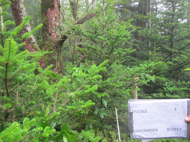
We pack our overnight gear into our backpacks, along with the tools of the monitoring trade – metal rebar, measuring tapes, hammers, nails, flagging, clipboards, and datasheets. Then we hit the trail at daylight. Today’s objective, Plot VSG362. That’s “Vital Signs – Greenbrier #362”, one of the 160 dots on the map that represent random plot locations for monitoring. These plots will be rectangles of forests that are marked with rebar stakes where we will collect data on forest growth, and return to periodically see how forests are changing. These locations run the gamut of Smokies forests: from high to low elevation, North Carolina to Tennessee. Once collected, data from these plots will give us a better picture on the health of our forests.

Though none of us have been to plot VSG362, we can see on the map that it’s somewhere in the saddle between Mount Guyot and Old Black, so we expect spruce-fir forests with dense growth of small trees. These forests were hit hard by a non-native forest pest, balsam woolly adelgid (Adelges piceae), in the latter half of the 20th century, which killed much of the Fraser fir (Abies fraseri).The increased sunlight on the forest floor has spurred thickets of regenerating fir and red spruce (Picea rubens) saplings.

Figure 2. A snapshot of plot VSG362, dense Fraser Fir saplings surround a mountain ash tree.

NPS Photo

After about two miles on trail, we prepare for the final bushwhack to the plot location. Lucky for us, the plot is only 50 meters off trail. However, the regeneration is thick and last night’s fog has left everything soaked. We’re at almost 6,300 feet elevation, where the vegetation is nearly always wet and hypothermia becomes a real threat - even in August. We suit up in rain gear under bright blue skies and charge in, following the GPS to the plot’s coordinates. Upon arriving at “Plot Center”, we are not disappointed. Today’s plot has sparse spruce trees over pockets of dead firs and thick regenerating saplings (Figure 2).

By this point in the summer, the crew is a well-oiled machine, and without much discussion everyone grabs their gear and begins installing the plot. We use measuring tapes and compasses to create a long rectangle in the forest, 20 meters wide by 50 meters long. At the corners and a few other strategic locations, we sink two-foot pieces of tagged rebar into the ground so that the exact same rectangle can be recreated in future years. We further divide the interior of the plot with measuring tapes into 10 different squares, 10 by 10 meters each. Due to the thick vegetation, it takes about two hours to get the plot set up, and then it’s time to get to work collecting data.

Figure 3. Park ecologist approaching a forest monitoring plot along the Appalachian Trail in a spruce/fir forest.

NPS Photo

Collecting Plot Data

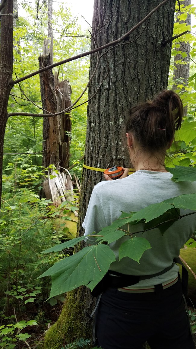
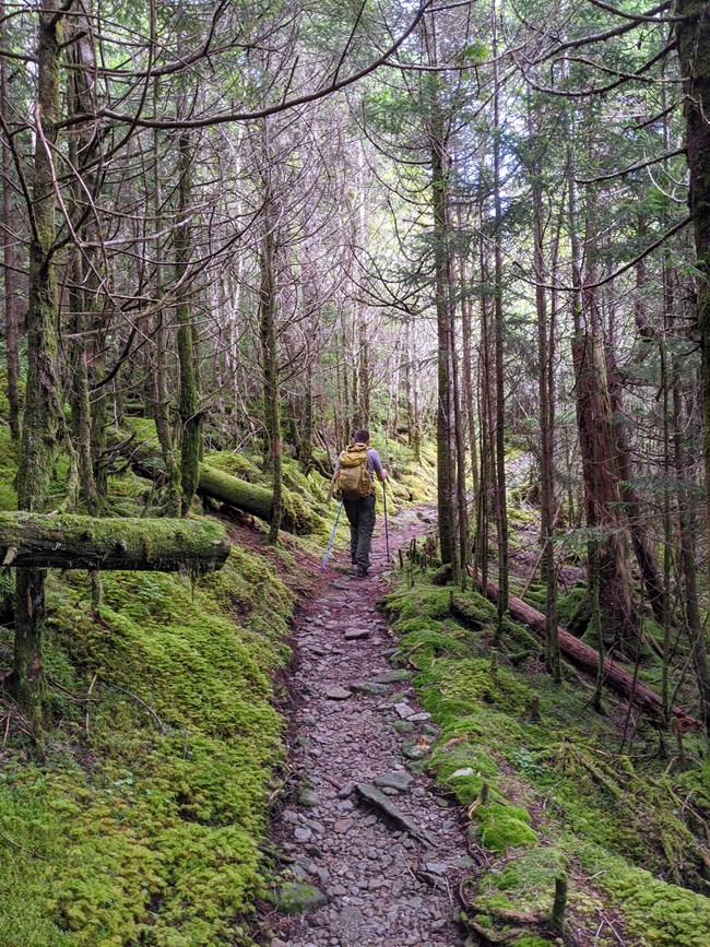
The crew divides into teams and begins working through the datasheets. A team of two identifies, measures, tags and maps overstory trees – today there will be 81 living trees and 57 dead trees to work through (Figure 1, following page). Another crew begins identifying and counting saplings, shrubs, and seedlings in smaller portions of the plot, then will take core samples from two trees using an increment borer. These measurements will tell us how this forest has and will continue to change. Counting tree rings on the cores, we will be able to understand how this forest has changed in the past. And we can understand the forest’s future potential based on the seedlings and saplings marching towards the canopy. That leaves a team of one, me, to create a full plant species list, collect soil samples and record environmental data such as slope, aspect, soil depth and canopy cover.

Progress is slow in this dense plot, and even with the early start to the day, we don’t finish until after lunch. The crew packs up the plot gear (minus the rebar stakes and tree tags, which are left in place) and is eager to get back on trail and out of their soaked rain gear. We have seven miles to go, down Snake Den Ridge Trail to our vehicle. We head down trail, naturally breaking into groups based on our hiking speed. As usual, I fall towards the back, preferring to move a little slower under the weight of an overnight pack (Figure 3). I enjoy good conversation with my crew members on the way down and think ahead to next week’s work. Plot VSG362 was the thirtieth plot of the year, leaving just two to go before the field season ends.

It will take five of these field seasons to collect data from all 160 plots. After that, we’ll start over again, collecting data from each plot for a second cycle. There is something reassuring about the thought of returning to VSG362 five years from now, almost like returning to your hometown after a few years away and driving around to see what’s changed. I’m sure a lot of the details from today will become hazy in my mind as time goes on and completed plots accumulate, but I know the data we collected today will always be there, a snapshot in time, to tell the story of this 20 x 50 plot of earth.

I shake my head and return to the conversation at hand. It’s the classic “What’s for dinner” conversation that happens so often in the last few hours of a multi-night backpacking trip. I remind myself that I’m lucky to work as part of a crew that I genuinely like spending time with, since we spend so much of it together this time of year. Just another day in the life of a forest ecologist.

A plot map of all overstory trees in plot VSG362.  Color, shape, and size represent tree species, diameter (cm) and live/dead status, respectively.  These maps will help to relocate trees in future resampling effort.

NPS Photo

More Information

Troy Evans, e-mail us

https://www.nps.gov/grsm/learn/scienceresearch.htm