
|
Geological Survey Professional Paper 1365
Ice Volumes on Cascade Volcanoes: Mount Rainier, Mount Hood, and Mount Shasta |
TABLE OF CONTENTS
Field measurements
Primary data reduction
Use of measuring point migration to correct for bedrock slope
Use of maps and photographs to infer basal topography
Ice-surface features and their relation to the basal topography
Isopach maps as interpretive tools
Determination of volumes
Measured glaciers
Unmeasured glaciers and snow patches
Results from four Cascade volcanoes
Mount Rainier
Mount Hood
Three Sisters
Mount Shasta
Appendix on monopulse radar
Application
ILLUSTRATIONS
PLATES 1-6. Maps showing: (omitted from the online edition)
1. Basal and surface contours of radar-measured glaciers on Mount Rainier, Washington.2. Isopachs of radar-measured glaciers on Mount Rainier, Washington.
3. Basal and surface contours of radar-measured glaciers on Mount Hood, Oregon.
4. Basal and surface contours of radar-measured glaciers on Three Sisters, Oregon.
5. Isopachs of radar-measured glaciers on Three Sisters and Mount Hood, Oregon.
6. Basal and surface contours of radar-measured glaciers on Mount Shasta, California, and Whitney Glacier isopachs.
FIGURE
1. Index map showing locations of volcanoes in study areas2. Photograph showing ice radar equipment used during study
3. Scheme of interactive processes to produce basal maps
4. Diagrams showing (A) location of transmitter and receiver and (B) slope correction necessary for measuring vertical ice thickness
5. Photographs of (A) Nisqually Glacier, 1944, and (B) Nisqually Glacier, 1980
6. Rock avalanche debris concealing glacier ice on Lost Creek Glacier, South Sister, Oregon
7. Diagram of a volume element
8. Photograph of Mount Rainier, Washington
9—11. Mount Rainier graphs showing:
9. Ice and snow area by altitude10. Ice volume by altitude on glaciers measured with ice radar
11. Ice area by thickness
12. Photograph of Mount Hood, Oregon
13—15. Mount Hood graphs showing:
13. Ice and snow area by altitude14. Ice volume by altitude on glaciers measured with ice radar
15. Ice area by thickness
16. Photograph of the Three Sisters, Oregon
17—19. Three Sisters graphs showing:
17. Ice and snow area by altitude18. Ice volume by altitude on glaciers measured with ice radar
19. Ice area by thickness
20. Photograph of Mount Shasta, California
21—23. Mount Shasta graphs showing:
21. Ice and snow area by altitude22. Ice volume by altitude on glaciers measured with ice radar
23. Ice area by thickness on Whitney Glacier
24—27. Diagrams showing:
24. Schematic of radar system25. Antenna detail
26. Oscilloscope output
27. Typical antenna configurations
TABLES
2—5. Areas and volumes of glacier ice and snow on:
2. Mount Rainier3. Mount Hood
4. Three Sisters
5. Mount Shasta
|
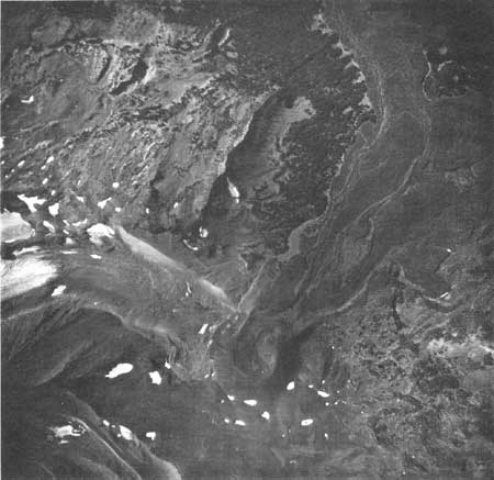
| Aerial photograph of Collier Cone, Oreg. (bottom-center of photograph), a cinder cone similar in eruption characteristics to the Mexican volcano Paricutin. Active between 500 and 2,500 years B.P. (Taylor, 1981, p. 61), the cone erupted between the lateral moraines of Collier Glacier. During the early 1930's, the terminus of Collier Glacier abutted the south flank of Collier Cone, reworking the cinders into the striated pattern visible today (Ruth Keen, Mazamas Mountaineering Club, oral commun., 1984). Williams (1944) reported the presence of glacial moraine interspersed with lava flows around the base of Collier Cone. (U.S. Geological Survey photograph by Austin Post on September 9, 1979.) |
DEPARTMENT OF THE INTERIOR
DONAL PAUL HODEL, SecretaryU.S. GEOLOGICAL SURVEY
Dallas L. Peck, DirectorLibrary of Congress Cataloging-in-Publication Data
Driedger, C. L. (Carolyn L.)
Ice volumes on Cascade volcanoes.
Supt. of Docs. no: I 19.16:1365
1. Glaciers—Cascade Range—Measurement. 2. Snow—Cascade Range—Measurement. 3. Volcanoes—Cascade Range. 4. Flood forecasting—Cascade Range. I. Kennard, P. M. (Paul M.) II. Title.
GB2420.D75 1985 551.3'1'09795 84-600381
SYMBOLS AND ABBREVIATIONS
| Symbol | Name |
| A | Surface area |
| b | Slope of bedrock measured from horizontal |
| c | Speed of light in ice |
| c0 | Speed of light in a vacuum |
| CI | Contour interval |
| d | Transmitter-receiver separation distance |
| g | Gravitational acceleration |
| h | Thickness measured perpendicular to the reflecting point on a glacier bed |
| h' | Vertical distance between the measurement point and the bedrock |
| i | (Subscript) indicates an interval value |
| k1,2,3 | Coefficients derived from regression analysis |
| l | Glacier length |
| p | Path of light |
| R | Resistance per unit length |
| t | Time between arrivals of air and reflected waves on the oscilloscope |
| V | Volume |
| V* | Volume estimation by calculation of basal shear stress |
| x | Distance from antenna feedpoint in meters |
| α | Slope of ice measured from horizontal |
 | Antenna half-length (meters) |
| η | Refractive index of ice |
| υ | Frequency |
| ρ | Density of ice |
| τ | Basal shear stress |
| τ* | Estimated basal shear stress |
| ψ | Resistive loading constant (ohms) |
CONVERSION FACTORS
For readers who prefer International System (SI) units, conversion factors for terms used in this report are listed below. Except where required by use with maps, stresses are expressed in bars (105 Pascals), a preferred unit in glaciology.
| Multiply inch-pound unit | By | To obtain SI unit |
| foot (ft) | 0.3048 | meter (m) |
| square foot (ft2) | 0.0929 | square meter (m2) |
| cubic foot (ft3) | 0.0283 | cubic meter (m3) |
| mile (mi) | 1.609 | kilometer (km) |
| square mile (mi2) | 2.590 | square kilometer (km2) |
| cubic mile (mi3) | 4.168 | cubic kilometer (km3) |
| pounds per square foot (lb/ft2) | 4.787 x 10⁴ | bar |
| slugs per cubic foot (slug/ft3) | 1.187 | kilogram per cubic meter (kg/m3) |
Water equivalence:
| Volume of water in cubic feet = | Volume of ice in cubic feet (1.8 slugs/ft3) 1.94 slugs/ft3 |
In this study, inch-pound units have been used to be compatible with the most current U.S. Geological Survey topographic maps.
| <<< Previous | <<< Contents >>> | Next >>> |
pp/1365/contents.htm
Last Updated: 28-Mar-2006