|
MESA VERDE
Environment of Mesa Verde, Colorado Wetherill Mesa Studies |

|
Chapter 2
design of the study
The scientific program of the Wetherill Mesa Project as envisioned by the project's supervisor, Douglas Osborne, included not only comprehensive archeological investigations on Wetherill Mesa but studies of the total environment of the Mesa Verde area. One approach in the latter range of studies was to obtain and compare precise quantitative data on selected environmental factors at sites that differed from one another in elevation or topography, over a period of at least 2 years. Such data on the present environment, it was reasoned, would contribute to studies of possible changes in the environment of the past, and ultimately lead to a fuller understanding of the prehistoric occupation of the area.
Since the Institute of Arctic and Alpine Research had operated an environment measurement program on the eastern slope of the Front Range in Colorado for 9 years (Marr, 1961), Osborne invited Marr and the Institute staff to plan the study, select and install the instruments, and provide technical supervision of the operation. Two of the authors, Erdman and Douglas, ecologists on the Wetherill Mesa Project staff, serviced the instruments and processed the data. As the study progressed, they made numerous improvements in the initial design and procedures. Other Wetherill Project personnel contributed in a variety of ways.
Harold C. Fritts of the Laboratory of Tree-Ring Research, University of Arizona, worked out, with Osborne, a dendroclimatological study to be integrated with the environment program. Its objective was to provide a basis for using tree rings as indicators of past climates (Fritts, Smith, and Stokes, 1965).
Six sites were chosen as samples of the environment gradient induced by changes in elevation along the tops of the mesas and by differences in topography within the canyons. The mesa-top sites were on Chapin Mesa and Park Point, and the canyon sites were in Navajo Canyon to the west (fig. 1). These sites, rather than sites on and adjacent to Wetherill Mesa, were chosen because of their accessibility to year-round visitation.
| Station | Elevation, feet |
Location |
| M—1 | 6,650 | Near the south end of Chapin Mesa. |
| M—2 | 7,150 | About 5 miles north of M—1 and near park headquarters. |
| M—3 | 8,575 | About 5 miles north of M—2 on Park Point, the highest point of Mesa Verde. |
| C—1 | 6,500 | West-southwest exposure slope. |
| C—2 | 6,382 | Canyon floor directly below and between C—1 and C—3. |
| C—3 | 6,500 | Directly opposite C—1 on northeast exposure slope. |
We studied stand ecosystems (Marr, 1961) and collected information on the vegetation and soil as well as the weather. Since organisms, environment factors, and processes are interrelated, by knowing one an estimate can be made of the other components. For example, an area with vegetation and soil similar to our C—1 station probably has a similar total environment.
ENVIRONMENT FACTOR MEASUREMENTS
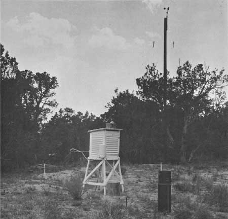
Measurements were taken from September 1961 through December 1963. The main body of data deals with solar radiation, air and soil temperature, precipitation, relative humidity, evaporation, wind, and soil moisture. In addition, at each station during the weekly servicing visit, observations were made on the type and amount of cloud cover, wind direction and velocity, and the depth and extent of snow cover. Stations were located in clearings where the effect of vegetation on the factors measured would be minimal. The hygrothermographs and recording units of soil thermographs were in a standard Weather Bureau cotton region-type instrument shelters, with the floor about 4 feet above ground in each instance (fig. 2). The shelters were erected in the summer of 1961 and dismantled in the spring of 1964 after our study was completed.

|
| Fig. 2 Recording instruments at M—2. Within the shelter are a hygrothermograph a 3-pen mercury thermograph, and maximum-minimum thermometers. On the roof is a pyrheliometer, and mounted on the side is an atmograph. |
The environment factors, except soil moisture, and the instrumentation for them are listed below:
| Factor | Instrument | Station | Recording |
| Solar radiation | Belfort pyrheliometer | M—2 and C—2 | Continuous. |
| Air temperature | Belfort hygrothermograph | M—2, M—3, C—1, C—2, and C—3 | Do. |
| Bendix-Friez hygrothermograph | M—1 | Do. | |
| Soil temperature at 2, 6, and 12 inches | Kahl 3-pen remote sensing mercury thermograph. | All stations | Do. |
| Precipitation | Standard 8-inch diameter precipitation gage. | M—1, M—2, M—3, and C—2 | Weekly and monthly totals. |
| Relative humidity | Belfort hygrothermograph | M—2, M—3, C—1, C—2, and C—3. | Continuous. |
| Bendix-Friez hygrothermograph | M—1 | Do. | |
| Evaporation | Piche atmograph | M—1, M—2, M—3, and C—2 | Continuous from May through October. |
| Wind | Bendix-Friez or Belfort 3-cup totalizing anemometers. | M—1, M—2, M—3, and C—2 | Weekly and monthly totals. |
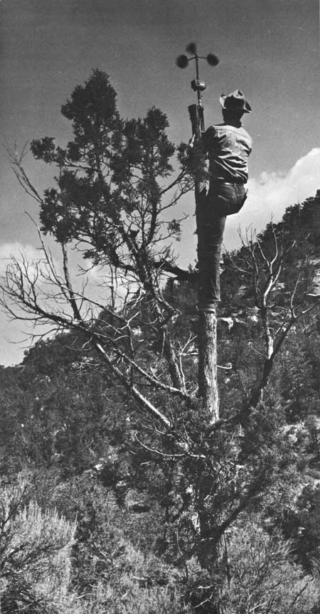
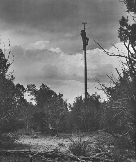
The pyrheliometer was mounted on the top, and the atmograph was attached to one side, of each shelter. Rain gages were mounted on individual supports with their rims about 4 feet above the ground. Anemometers were mounted on a tree (fig. 3) or on utility poles (figs. 4 and 5), so that the instruments were several feet above the general level of tree crowns. Soil samples for gravimetric measurement of water content were collected at the edges of the clearings.
|
| Fig. 3 A 3-cup totalizing anemometer atop tree at the canyon-bottom site. |
|
| Fig. 4 The juniper-pinyon/bitterbrush community characteristic of M—1, near the southern end of Chapin Mesa, at 6,650 feet elevation. The 30-foot anemometer support indicates the stunted nature of the trees, their height ranging from 15 to 20 feet. Note the paucity of the understory. |
|
| Fig. 5 M—2, near park headquarters on Chapin Mesa, at 7,150 feet elevation, looking southwest. Note pioneer vegetation on the abandoned dirt tennis court. |
The Piche atmograph records evaporation from a standard 5.0 cm. filter disk provided with a continuous supply of distilled water; during dry intervals of high evaporation, we substituted 3.0 cm. filters. Wet and dry bulb temperatures were determined with a Bendix motor-aspirated psychrometer at each station visit when humidity was reasonably stable. These data verified the accuracy of the hygrograph record. Weather Bureau-type maximum and minimum thermometers mounted on the inside wall of the instrument shelter were read and reset at each servicing; these data gave a check on the accuracy of the thermograph trace. As a check of accuracy for the soil thermographs, a Kahi asphalt-type skewer thermometer was periodically inserted to the depth of each soil-temperature sensing unit.
Some difficulties were encountered over which we had no control. In spite of careful tests in the laboratory prior to installation, the M—2 and C—3 soil thermographs went out of adjustment for short periods, the M—2 instrument during the fall of 1962 and the C—3 instrument during November and December 1962. Also, recent calibration tests of the pyrheliometers suggest that although the instruments were in excellent agreement with one another the values recorded may have been higher than those which actually occurred.
The stations were serviced each week and on the last day of each month, all stations being visited on the same day except when adverse weather precluded this. Erdman or Douglas evaluated the raw data of each servicing in search of possible errors. Any adjustments indicated were recorded on the original data sheet or chart. Laboratory assistants transferred the data to initial summary tables. In the case of solar radiation, this task involved measurement of the area under the daily traces on the pyrheliograph chart with a compensating polar planimeter. This area under the curve was then converted to a gram calorie unit (gm. cal./cm.2/day) by computer at the Numerical Analysis Center at the University of Arizona.
Correctness of the data transfer was insured by two laboratory assistants working together, one reading the original data and the other checking figures on the data transfer sheet. The initial data summaries were transferred to IBM punch cards at the Numerical Analysis Center. An IBM 1401 program, produced by Robert Baker, computed the daily means, monthly totals, and monthly averages, and printed the monthly summary tables. At Mesa Verde, annual summaries (see appendix) were compiled from the monthly summaries.
The summaries were checked by Marr and Institute assistants by comparing the data from the different stations and tracing apparently odd relationships back to the original data. (The original charts and printed and punched monthly summaries are filed at the Institute of Arctic and Alpine Research and are available for study by interested scientists.)
Soil Studies
The descriptions of soil profiles used in this report were supplied by Orville A. Parsons. The soil moisture constants of percent moisture at 1/3 and at 15 atmospheres (field capacity and permanent wilting percentage equivalents, respectively) were determined by pressure membrane techniques for soils collected at each station. The samples were collected and screened through a 2 mm. sieve at Mesa Verde. Measurements were made by the Department of Agronomy, Colorado State University, Fort Collins.
In order to determine how much the moisture tension values were in accord with the actual permanent wilting points of these soils, wheat seedlings were planted in four replicate samples of the soils from stand M—2, and the soils were allowed to dry until permanent wilting was reached. The percentage of moisture was then determined for each sample. The following results show the close agreement between the pressure membrane method and the seedling wilt method:
| Sample depth | 15 atmospheres | Permanent wilting point | ||
| Percent moisture | Range | Percent moisture | Range | |
| 2 inches | 7.1 | 2.2 | 7.5 | 2.2 |
| 6 inches | 10.6 | 5.2 | 10.6 | 1.2 |
| 12 inches | 9.3 | 2.2 | 9.8 | 2.5 |
Vegetation Studies
Native vegetation is regarded as the best expression of the totality of a climate. Koppen selected many of his climate boundaries with vegetation limits in mind (Trewartha, 1954, p. 225). The understory and, indeed, the appearance of the trees themselves serve as valuable indicators of the local environment.
Erdman studied the vegetation of each stand, using the point quarter method of Cottam and Curtis (1956) for features of mature trees, and ten 4- by 50-foot belt transects spaced at 25-foot intervals for tree reproduction data. Categories used in the reproduction study were: seedlings = less than 1 foot high; saplings = stems less than 2 inches in diameter; trees = stems more than 2 inches in diameter. A list was made of species observed in each community (see ch. 3, table 2), using the nomenclature in the checklist by Welsh and Erdman (1964), with certain up-to-date changes furnished by William A. Weber. Increment cores were collected from representative pinyons to get an estimate of the age of the stands. Dating of these samples was done according to the Douglass system (Glock, 1937).
Ages of the mature junipers could not be determined because of lobing and erratic growth.
| <<< Previous | <<< Contents>>> | Next >>> |
archeology/7b/chap2.htm
Last Updated: 16-Jan-2007