MOUNT RAINIER The Forest Communities of Mount Rainier National Park

Our general methodology was essentially the same as that widely applied in forest classification in the western United States (Pfister and Arno 1980) and in the USDA Forest Service Area Ecology Program (see, e.g., Henderson and Peter 1981). More comprehensive discussions of the philosophy underlying such studies can be found in these and related references.

Field Sampling

Our sampling was designed to cover the full range of forest types in all sectors of the Park and throughout each forest zone. Stands were sampled, therefore, by a reconnaissance technique modified from Dyrness et al. (1974). The field crew traveled a slope, trail, road segment, or path through the forested landscape and established a sequence of sample plots that revealed both typical and changing forest patterns. Whenever major changes in dominance relationships of tree or understory vegetation were observed along these routes, the crew would look for a forest stand of sufficient size and homogeneity to establish a sample plot. The plots were usually circular and 500 or 1000 m² (0.125 or 0.25 acre) in size, depending on the densities of the larger sized trees. Additional plots from Franklin's (1966) earlier study were included. Stands ranged in age from about 70 years to over 1,000 years since major disturbance, but all presented essentially a forest environment mostly characterized by a closed or semiclosed tree canopy. In some places, especially at higher elevations or on more exposed sites, the field crew sampled more open forests if understory vegetation generally resembled that of closed forests. A total of 518 plots provided the basis for the classification presented here.

In each circular plot, all tree stems exceeding 1.4 m (4.5 ft) in height were tallied by species and diameter at breast height (d.b.h.) by diameter classes of 1-dm (4-in) intervals. We defined "established seedlings" as trees between 1 and 14 dm (4 and 55 in) in height, and counted these in either a 50-m² (545-ft²) circular plot at the center of the larger plot or at four 12.5-m² (136-ft²) circular plots in each quadrant of the larger plot.

Understory herbs and shrubs were recorded by the extent of their canopy coverage; this was estimated visually over the entire plot to the nearest percent for species with less than 10 percent cover, and to the nearest 5 or 10 percent for those with over 10 percent cover.

Soil types (Hobson 1976) and general morphological features were described from small pits (usually one per plot) located in areas of typical understory vegetation. Other environmental data collected at each plot included: elevation, exposure, slope, landform, position in landscape (lower, middle, upper slope, bench, ridge, valley), and location on a U.S. Geological Survey topographic map. Conspicuous or unusual features of forest stands were described as notes or remarks. These included evidence of fire, influence of animals, windthrow, mosaics, and ecotones with other forest types.

Stand ages were estimated from increment cores of dominant trees judged to be among the first wave of regeneration after disturbance. Rings from cored trees were counted in the field. Age was estimated from the ring count plus corrections for center and age-to-core height. Generally, the older trees of a cohort were sought in order to determine a time limit for whatever disturbance gave the opportunity to establish that cohort. When available, ring and age data from stumps or cut sections of tree falls along trails were also useful for estimating cohort ages.

Data Analysis

Our classification of the forests at Mount Rainier was an interactive procedure between plot sorting based on field judgments and data analyses and displays from a computer (Franklin et at. 1970, Pfister and Arno 1980). The first 400 plots were used in steps 1 through 10. Specific steps were as follows:

1. Initial synthesis tables were developed by manual sorting. At the end of each field season, plots were organized into tables according to dominant, diagnostic features of tree, shrub, and herb vegetation (Shimwell 1972). The major features we used were tree species present in seedling and sapling size classes and dominant shrub and herb species.

2. Data were coded, edited, and verified for computer processing. The entire data set was too massive for computer handling, so we simplified it for the initial analysis. For example, minor species (those that occurred in less than 1 or 2 percent of the plots) were excluded. Certain more common species not thought to have classificatory significance were also excluded. These were species with a wide ecological amplitude and low site indicator value, such as Epilobium angustifolium and Goodyera repens.

3. Environmental plot groupings were developed. Plots were assigned into four groups approximating the major environmental regimes of the forests at Mount Rainier (moist, modal, dry, and cold). Each group contained up to 125 plots, and doubtful plots were assigned to more than one group. Each group was subject to the similarity and principal component analyses described below.

4. Similarity matrices were computed for all plots for each environmental group. The index of similarity was that of program SI MORD (Dyrness et al. 1974)—a percentage similarity (Sorensen's index) based on dominance of selected tree and understory species. Species chosen for similarity computations were thought, in our judgment, to have possible classificatory significance by their restricted distributions. Different sets of species were used in each of the four groups.

5. Initial plot clusters were extracted. Highly similar plots representing typal communities (Daubenmire 1966) were sought from each group similarity matrix. Our field judgment and the initial groups (step 1) were necessary for the initial discrimination of these clusters of "modal plots." Generally the plot similarities within the initial clusters exceeded 30 and sometimes 40 per cent.

6. Diagnostic vegetative and environmental features of the modal plot clusters were identified and incorporated into abstracts of each tentative type.

7. Plot clusters were expanded. The modal plots of step 5 did not contain the full range of variation of forest vegetation or environments. The similarity matrix was further examined for unassigned plots having mostly intermediate similarities (20- to 30-percent) to plots of the modal clusters. The unassigned plots were classified into a forest grouping whenever the diagnostic or environmental features of the appropriate modal cluster (step 6) were satisfied. This step involved considerable ecological judgment for those plots having only weak expressions of the diagnostic criteria.

8. The reduced similarity matrix for ungrouped plots were examined for further typal communities. Steps 5-7 were repeated until a small residue of unassigned plots remained; these were considered intergrades or unclassifiable as unique stands.

9. Revised synthesis tables were constructed for the emerging similarity groupings. The similarity matrix was reorganized to display similarities in intergroupings and intragroupings. The stand tables and reorganized similarity matrix were then used to check for anomalous or misclassified plots and possible reassignment (Franklin et al. 1970, Pfister and Arno 1980). Again, field experience and subjective judgments were sometimes needed to confirm or change the assignment of plots difficult to classify. Plots that were typically difficult to assign were stands with depauperate understories as a result of dense tree canopies.

10. Principal component analysis (PCA) was carried out with species correlation matrices (R-matrix) computed within each environmental group (step 3) using the same classifier species characteristics employed for similarity analysis. The R-matrix was used for the axis extraction procedures of PCA (Cooley and Lohnes 1971).

11. Discriminant analysis was performed on 19 forest groups defined after step 9 was completed. Discriminating variables were selected among those species that had high values of importance in the initial stand tables of step 1; 39 species were used. Discriminant functions were computed by procedures described in the "Statistical Package for the Social Sciences" (Nie et al. 1975) to optimize separation of the 19 groups in multivariate space. To provide an independent test of the classification, over 100 additional plots (plot nos. 401-518), which had never been used in the analysis to this point, were classified according to the discriminant functions. In an additional test, all of the plots already assigned to forest groups by similarity procedures (step 9) were subjected to discriminant analysis. This reexamination revealed less than 5 percent of the plots had a high probability of misclassification. Such plots were reexamined and, when warranted by ecological judgment based on information not used in discriminant analysis (such as soil type), were either reassigned to another forest type, kept in the assigned type, or not classified.

12. Once step 11 was completed, the final synthesis and summary tables were prepared using all 518 plots. Synthesis tables were printed by computer for the full set of data for each forest type. The printouts also tabulated slope-corrected densities for established seedlings, saplings (0-20 cm or 0-8 in d.b.h.), poles (20-50 cm or 8-20 in d.b.h.), and standards (d.b.h. over 50 cm or 20 in). Tree densities by 10-cm (4-in) d.b.h. size classes and basal area were also printed for every plot within each forest type (trees over 120 cm or about 50 in d.b.h. were printed individually). Canopy coverage of understory shrubs and herbs (arranged alphabetically) were tabulated by plot. These tables are on file at the Forestry Sciences Laboratory, Corvallis, Oregon, and at the headquarters of Mount Rainier National Park.

We also prepared a directory of plots and summary tables for each forest type, except for several minor types. The directory tabulates location and environmental data for each plot and provides a listing of plots within each forest type. The summary tables contain data averaged over all plots within each forest type. Summaries for trees include slope-corrected densities and basal areas. Summaries for major or descriptive shrubs or herbs (106 taxa are tabulated) include constance (the percentage of plots containing a taxon) and percent canopy cover (averaged over all the plots within each forest type and not just over plots on which it occurred). Total shrub and total herb cover percents are the sums of the average cover percent for tabulated shrub and herb species (the nontabulated understory plants contribute little average cover to the forest types).

The entire plot data set is available at cost on magnetic tapes from the Forestry Sciences Data Bank, Forest Science Department, Oregon State University, Corvallis, Oregon 97331.

Terminology and Nomenclature

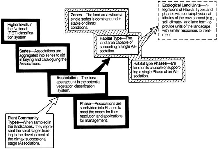
Our classification uses terms now standardized in the western United States (Daubenmire and Daubenmire 1968, Pfister et al. 1977, Pfister and Arno 1980, Layser and Schubert 1979, Henderson and Peter 1981). This discussion of the vegetative classification hierarchy is taken largely from Henderson and Peter (1981). The major units of interest to us are plant community type, plant association, plant series, and habitat type (Fig. 10). Plant community types are aggregations of plant communities (the actual stands observed and sampled in the landscape) that are judged to be very similar based upon analyses of the type outlined in the previous section. When a plant community type is based upon mature or old-growth stands and emphasizes the stable or potential climax components, it is termed a plant association. The plant association is, then, a special type of plant community, i.e., a climax plant community. Plant associations can be aggregrated into plant series (Fig. 10) which, in forests of the western United States, turn out to be groupings of plant associations with the same dominant climax tree species. Geographic varieties of a major plant association are sometimes recognized as phases. The plant association characterizes a particular kind of environment and can therefore be used as a basis for distinguishing land areas of differing environments and biological potential. All of the land area capable of supporting the same plant association or climax vegetation is called a habitat type (Fig. 10). The habitat type is named for its potential vegetation, a practice which sometimes leads to a confusion between something which is a plant community type (association) and an actual land area which may or may not currently be occupied by that vegetation. A zone has the same relation to habitat type that series has to plant association.

Figure 10. The classification hierarchy (from Henderson and Peter 1981). (click on image for an enlargement in a new window)

The final synthesis tables (see step 12 in the previous section) provide the basis for identifying the major forest communities in Mount Rainier National Park. Fourteen of these communities are plant associations based upon mature and old-growth forest stands. We considered mature forests to be 200 years or more in age and in which (1) tree population structures suggest the ultimate climax species composition and (2) the understory is relatively stable, at least in dominance relationships among the major species. Associations are sometimes divided into phases to reflect minor but consistent geographic, environmental, and floristic variations in the basic type. Obviously, a plant association can be used to distinguish land areas of similar ecologic potential, i.e. a habitat-type, and, as mentioned, the habitat type is named for its distinguishing (but sometimes absent) plant association.

Some early successional or young stands could not readily be related floristically or environmentally to plant associations. Consequently, five community types are identified in our Mount Rainier classification. These types represent the most general level in the hierarchy (Fig. 10); they are immature, unstable communities and are expected to evolve into one or more of the plant associations over time. The value of these communities as environmental indicators is obviously limited and they do not distinguish a habitat type.

The emphasis on older forest stands and potential vegetation (plant associations) is because of their value as indicators of environmental conditions. Early successional species, including seral tree species, are commonly generalists with broad ecological amplitudes. Later successional species tend to be much more attuned to local environmental conditions and have, therefore, much greater value in locating oneself on an environmental field (see, e.g., Zobel et al. 1976).

Nomenclature of each plant association is typically a binomial. The first name consists of a leading climax tree or sometimes a leading associated late seral or co-climax tree. The tree portion of the name is followed by a slash, then by a major, diagnostic understory species. Community types were named by the leading seral tree, followed next by a slash, then by a major diagnostic understory species. In many illustrations and tables we have used abbreviations for the species that comprise the names of habitat and community types. These abbreviations are defined on the inside front cover.