The National Park Service's History Program was started in 1931 and is managed by the Chief Historian of the National Park Service. It administers multiple program areas, conducts historical research, and supports National Park Service staff in all matters relating to the Service's history and mission.
Administrative History Program
Provides guidance to NPS parks, programs, and regions writing new administrative and legislative histories or updating existing histories.
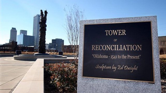
African American Civil Rights Network
Commemorates, honors, and interprets the history of the African American Civil Rights movement.

American World War II Heritage City
Honors communities and their citizens who supported America's war effort on the home front.
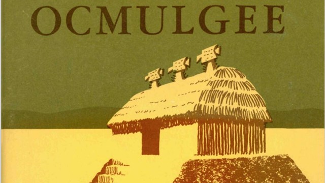
Classic NPS Publications Series
Handbooks and proceedings created for park staff, researchers, professionals, students, and the public.

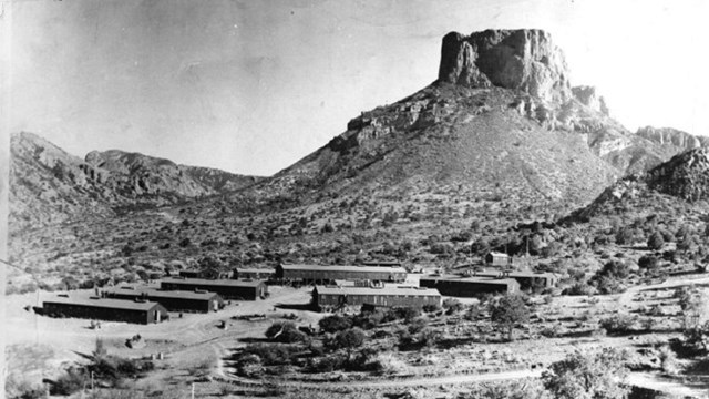
Historic Resource Studies
Provides an historical overview of a park or region and inventories and evaluates their historic resources.

History of the National Park Service
A collection of digital resources that offer insights into the history and growth of the National Park Service.

Maritime Heritage Program
Administers the National Maritime Heritage Grants and also helps to document and protect historic maritime resources.

National Historic Lighthouse Program
Allows historic light stations to be transferred at no cost to federal agencies, state and local governments, nonprofits, and others.

Oral History Program
Uses in-depth interviews to document the history of the National Park Service. Provides guidance and help to park units and programs.

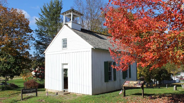
Park National Register Documentation
Works with NPS staff to list national park units and their historic resources in the National Register of Historic Places or as NHLs.
Special History Studies
Studies that focus on the history of specific topics, themes, resources, or time periods.

America 250
Opportunities to celebrate, commemorate, and contemplate the upcoming 250th anniversary of the signing of the Declaration of Independence.
Last updated: May 7, 2024