Geological Survey Professional Paper 516—E A Geophysical Study in Grand Teton National Park and Vicinity, Teton County, Wyoming

FIELD MEASUREMENTS

Some gravity survey work was done in the mapped area in 1955 by Lavin and Bonini (1957), of Princeton University. From their base station, which was tied to gravity station GW35 at Billings, Mont. (Behrendt and Woollard, 1961), they established 280 field stations. In 1964-65, Behrendt, during the present investigation by the U.S. Geological Survey, established 430 additional stations. The survey was tied to the North American gravity-control network by means of LaCoste and Romberg geodetic gravimeter G—8. A base station at Jackson Airport was tied to station WU7 at the Colorado School of Mines, Golden, Colo. (Behrendt and Woollard, 1961). Reoccupations by the Geological Survey of the earlier Princeton University base station showed a difference of only 0.1 mgal (milligal) between the two surveys. Because the data were contoured at a 5-mgal interval, this difference was neglected. Worden gravimeters W226, W177, WE134, and W57 were used for the survey; W57 was calibrated against a portion of the North American calibration range, and for the other gravimeters the manufacturer's calibration was used. Elevations were obtained from bench-mark data, spot elevations on topographic maps, and barometric altimetry. The elevations are accurate to 1-2 m in the areas of low relief, for which modern maps were available; but they may be in error by as much as 10-20 m in areas of high relief, such as the Teton Range, for which modern maps were not available. These greater errors correspond to 2- to 4-mgal errors in the Bouguer anomalies. On Jackson Lake, stations were observed on ice, and water depths were obtained by echo sounding and from an unpublished bathymetric map of the National Park Service. Terrain corrections were made out to Hammer Zone M, except for the highest stations for which corrections were carried out to a distance where they became negligible. A density of 2.67 g per cm³ (grams per cubic centimeter) was used in the Bouguer reduction. The gravity results are shown on plate 1, which also shows the generalized geology by Love (1956c) and John C. Reed, Jr. (unpub. data). Love's (1956b) tectonic map of Teton County is shown in figure 2. Other gravity surveys in adjacent areas have been published by Bonini (1963) and by Pakiser and Baldwin (1961).

Four seismic refraction experiments were made in 1964 and 1965 to study the seismic velocity structure in Jackson Hole. The objective was to correlate the information thus obtained with the gravity and geologic data and thereby gain an understanding of structural relationships in the region. The locations of the four profiles are shown on plate 1. Each array in 1964 consisted of six geophones located at 0.5-km intervals. The one array used in the 1965 experiment consisted of 12 geophones spaced 0.2 km apart. In places where the configuration was not in a straight line (pl. 1), lateral homogeneity was assumed. Charge size ranged from 3 to 300 kg (kilograms). Arrival times are accurate to ±0.01 sec (second), and distances are accurate to ±100 m. Elevation corrections were not made for lines 1-3, which cover terrain whose maximum relief was about ±30 m (about ±0.01 sec). Elevation corrections were made for traveltimes on line 4, where relief was as much as 130 m.

An aeromagnetic survey was flown at a constant barometric elevation of 3,700 m, except that the elevation was 4,300 m over the high peaks of the Teton Range. The north-south flight lines were spaced 1.6 km apart. The results of the survey are shown on plate 2, together with part of an unpublished aeromagnetic survey of Yellowstone National Park. A residual map, constructed by removing the earth's field linearly as shown by the total intensity map of the United States for 1965 (U.S. Coast and Geod. Survey, 1965), is shown on plate 3. All estimates of depth to sources of magnetic anomalies were calculated by the method of Vacquier, Steenland, Henderson, and Zietz (1951) with the observed profiles. The exclusive use of this method is justified by the ruggedness of the topography, which would make more sophisticated computations unrealistic.

GRAVITY SURVEY

The Bouguer anomaly map (pl. 1) shows several interesting features. The most apparent is the —240-mgal negative anomaly over Jackson Hole compared with —185 mgal over the Teton Range. A steep gradient, clearly associated with the Teton fault near the south end of the range, broadens northward near Jenny Lake and trends north-northeast across the lake. The gradient steepens considerably below the northeastern part of Jackson Lake, reaching a maximum of 15 mgal per km (milligals per kilometer) near Arizona Creek. The Teton fault (pl. 1; fig. 2) was drawn to conform to the steep gravity gradient. The 55-mgal anomaly results from contrast between low-density sedimentary rock in the basin and relatively high-density Precambrian crystalline rock of the Teton Range.

The most negative parts of the Bouguer anomaly map coincide with the area of thickest low-density Tertiary and upper Mesozoic sedimentary deposits, which is near the east edge of Jackson Lake. Thick low-density deposits also occur just north and south of Blacktail Butte and south of Jackson.

The west-northwest trend of the Gros Ventre Range, which is reflected on the gravity map, appears to influence the gravity contours in the southern part of the Teton Range, as might be expected from the relative ages of the two uplifts (table 1). Blacktail Butte is associated with a 10-mgl positive anomaly caused by the density contrast between the relatively dense Paleozoic rocks and the less dense Tertiary sedimentary rocks.

The saddle between the —225-mgal contours between shotpoints 2.2 and 2.3 indicates a relatively broad anticline as discussed on page E19.

The extrusive volcanic rocks in the northern part of the area do not seem to have a great effect on the Bouguer anomalies, a condition that suggests that the rocks are of low density contrast or that they are thin; probably they are both.

Because of uncertainties about elevation, the significance of anomaly closures shown within the Teton Range is difficult to evaluate. The contours at the north end of the range show 20 mgal of relief and reflect northerly anticlinal plunge of the crystalline core of the range.

SEISMIC-REFRACTION SURVEY

PROFILES 1-3

SLOPING LAYER ANALYSIS

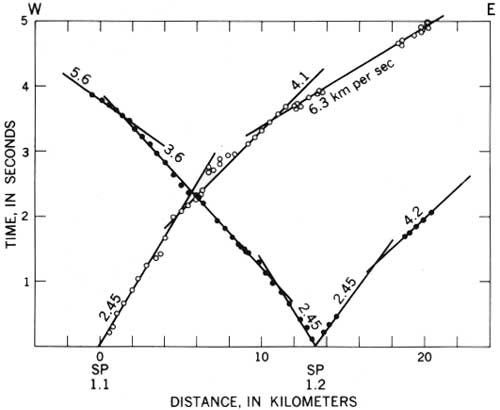
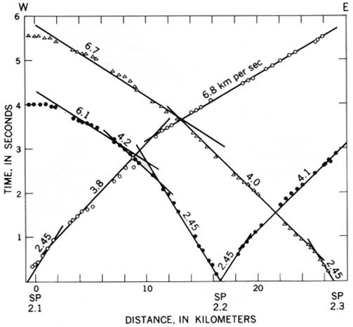
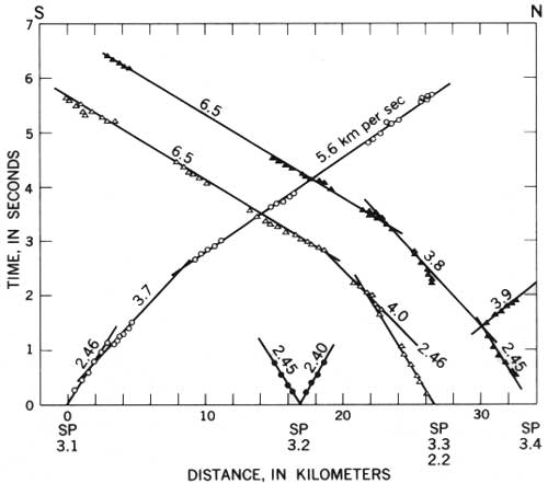
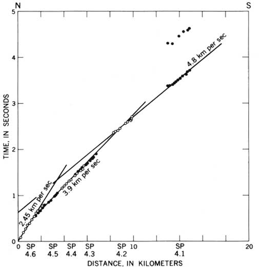
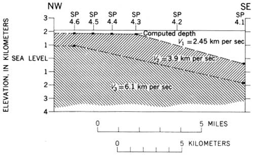
The seismic velocity structure within the sedimentary rock and crystalline basement underlying Jackson Hole was studied by refraction methods. Three observed profiles are located on plate 1, and data on their travel times are shown in figures 3-5. Lines 1 and 2, as planned, gave maximum structural control, and line 3, which was laid out along the strike of the gravity minimum, gave the best velocity information. Note the early arrival data from the 6.1-km per sec (kilometers per second) apparent velocity at the west end of line 2 (fig. 4); there the line crosses the Teton fault area (pl. 1). A three-layer model (fig. 6), based on the apparent velocities shown in figures 3-5 and using a critical distance analysis for sloping layers, gives a good fit to these data. This model, because it was constructed on the basis of the apparent velocity lines (figs. 3-5), does not show that the Teton fault crosses the profile east of 2-1, whereas the traveltime curve (fig. 4) and the gravity data (pl. 1) indicate that it does.

FIGURE 3—Seismic traveltime graph for line 1. Apparent velocities, in kilometers per second, are shown. SP, shot-point.

FIGURE 4.—Seismic traveltime graph for line 2. Apparent velocities, in kilometers per second, are shown. SP, shot-point.

FIGURE 5—Seismic traveltime graph for line 3. Apparent velocities, in kilometers per second, are shown. Shot at 3.2 had insufficient energy. SP, shotpoint.

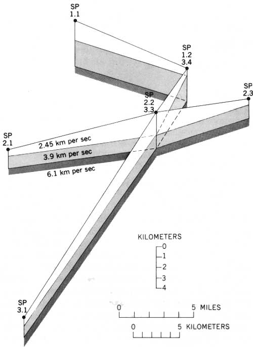
FIGURE 6.—Sloping layer model fitted to traveltimes for seismic lines 1-3. SP, shotpoint.

The thickest parts of the 2.45 km per sec layer are at shotpoints 1.1 and 2.2-3.3, where gravity values are lowest. Model depths to the 3.9 layer arc 1.5 and 1.4 km, and depths to 6.1 are 3.2 and 2.7 km, at shot points 1.1 and 2.2-3.3, respectively.

DELAY TIME ANALYSIS

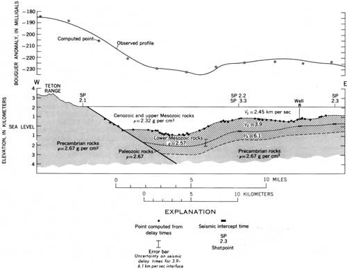
The traveltime data show considerable scatter from the apparent velocities shown in figures 3-5, which is the result of departures from the uniform velocity-planar interface assumption of the model shown in figure 6. On the assumption that the scatter is the result of variations in the thickness of the layers, and that the three velocities of the sloping layer model are real, a delay time analysis was made of line 2 using the method of Pakiser and Black (1957). The interface calculated at the base of the 2.45-km per sec layer and the scatter are shown in figure 7. The analysis for the 3.9- to 6.1-km per sec interface, because of cumulative errors, was much poorer than that for the 2.45-km per sec interface (fig. 7). The estimate of the uncertainty of this surface is represented by the error bar shown in figure 7. The depth at shotpoint 2.2-3.3 was used as a tie point for the base of the 2.45-km per sec layer, and the depths at 2.2-3.3 and 2.3 were used for the contact between the 3.9- and 6.1-km per sec layers.

FIGURE 7—Seismic delay-time model for seismic line 2. Bouguer gravity-anomaly curve is compared with theoretical (computed) points computed from seismic model by the two-dimensional line integral method using densities shown and a regional slope of —0.72 mgal per km to the east. Standard deviation of computed points is ±2.0 mgal. (click on image for a PDF version)

The well shown in figure 7 is about 100 m north of line 2. This well penetrates the Cloverly Formation (Lower Cretaceous), in which the 3.9-km per sec refractor is interpreted to occur. The exposed Cloverly nearby is quartzitic (Love, 1956a), and it may be the top of the 3.9-km per sec refractor. Commercial seismic companies use this formation or its equivalent as a reflection marker horizon throughout Wyoming (Berg, 1961; Peters, 1960). A good reflecting surface suggests, although it does not prove, the presence of a good refractor. A velocity of 3.9 km per sec might be expected in Cretaceous sedimentary rocks (Blundun, 1956).

The 6.1-km per sec layer is interpreted to include both Paleozoic and Precambrian rocks (fig. 7). Because the Paleozoic section consists primarily of limestone and dolomite (table 1), a velocity of 6.1 km per sec is not improbably high; Blundun (1956) reported a Mississippian limestone in Alberta whose velocity was 6.4 km per sec.

The obvious alternative to this interpretation would be to accept the 6.1-km per sec refractor as the crystal line basement; however, this would leave no place for the Paleozoic rocks, for a kilometer of carbonates could not be accommodated in the 3.9-km per sec layer. It is unlikely that the Paleozoic rocks are absent in Jackson Hole, for they crop out in the surrounding mountains and in Blacktail Butte. Contact between the 3.9- and 6.1-km per sec layers, therefore, is placed at the top of the Paleozoic rocks.

The depth shown at the well (fig. 7) to the top of the Paleozoic rocks is interpreted from two wells in the Spread Creek area about 6 km to the south (Love and others, 1951); the extrapolated thickness of the Lower Cretaceous section probably does not vary more than about 100 m in this distance. The contact between the Paleozoic rocks and the Precambrian basement was not recognized in the refraction data, owing to the low velocity contrast (possibly even a reversal). Undoubtedly, the later arrivals on lines 2 and 3 are sufficiently distant from the shotpoints to have been refracted through a higher velocity at the Paleozoic-Precambrian contact, if one exists. In figure 7, the depth shown to this contact, at the well, is based on the thickness of the Paleozoic section in the Spread Creek area, and the dashed contact was drawn assuming constant thickness along the profile.

GRAVITY ANALYSIS ALONG LINE 2 PROFILE

The gravity analysis along the line 2 profile was based on a theoretical gravity profile of the seismic model which was calculated by use of the two-dimensional line integral method compared with the observed data (fig. 7). Density contrasts —0.35 and —0.1 g per cm³ for the 2.45- and 3.9-km per sec layers, respectively, relative to the 6.1-km per sec layer, with a regional gradient of —0.72 mgal per km to the east, gave the best fit to the observed data. The standard deviation of the computed points relative to the observed profile is ±2.0 mgal. The 2.45-km per sec layer, on which seismic control is the best, is the major influence on gravity variation in this profile as well as on the Bouguer anomaly map (pl. 1). Another gravity model calculated for the seismic model of figure 7, assuming only a density contrast of 0.4 g per cm³ between the 2.45- and 6.1-km per sec layers, gave nearly as good a fit with standard deviation ±3.1 mgal. This second calculation illustrates the degree to which the upper layer controls the gravity variations, but it is less plausible geologically than the model shown in figure 7.

The Teton fault is shown in figure 7 as an east-dipping normal fault. The shape of the contact between the Precambrian crystalline rocks of the Teton Range and the younger sedimentary rocks, calculated from the seismic data, does not indicate a steeply dipping fault. The computed gravity values are in agreement with the observed data, and even suggest that a slightly lower angle might give a better fit. The fault may be a single break of rather low dip, as shown in figure 7, or it may consist of several closely spaced more steeply dipping faults arranged steplike to the average slope. The main constraint in any such steplike arrangement is that the contact between the 2.45- and the 3.9-km per sec layers must remain nearly as shown in figure 7. The geophysical data do not discriminate between these possibilities, but the latter is favored as being more reasonable geologically. This analysis supports Love's (1956b) interpretation that the Teton fault is a normal fault.

The anticline mentioned previously (p. E16) as observed on the gravity map (pl. 1) is not shown in figure 2; but it is reflected in the contact between the 2.45- and 3.9-km per sec layers, and its axis appears to be near shotpoint 2.2-3.3 (pl. 1; fig. 7). In the area of the profile this anticline is more prominent than the Spread Creek anticline (Strickland, 1956), and the two are separated by a syncline. The Spread Creek anticline in the vicinity of the well (fig. 7) is barely recognizable in the seismic data, and its gravity effect is negligible.

PROFILE 4

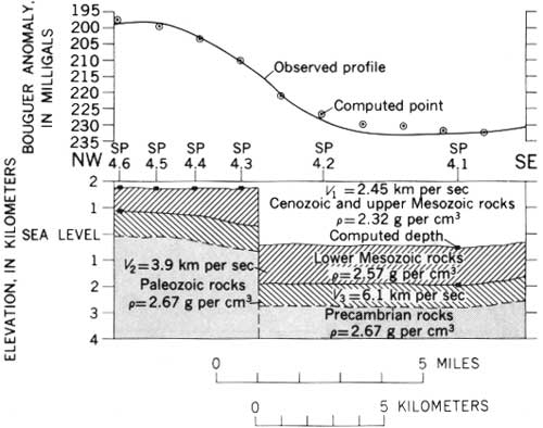
The steep gravity gradient observed along the northeast shore of Jackson Lake suggested that a branch of the Teton fault trends through this area and is steeper than along line 2. The seismic refraction experiment carried out along line 4 in 1965 (pl. 1) tested these inferences. The traveltime plot is shown in figure 8. The velocities determined for lines 1-3 were used, and traveltime variations due to structure were assumed. The arrivals from six shots were recorded at one location (pl. 1) consisting of a 12-geophone spread. Apparent velocities fitted to the data by the method of least squares were used to identify the arrivals. Thus, shot 4.6 was refracted through only the first layer, shots 4.5, 4.4, and 4.3 penetrated the second layer, and shots 4.2 and 4.1 reached the third layer. Good second arrivals through the second layer were also recorded from shot 4.1. The time-depth method of Hawkins (1961) was used to determine the depth of the 2.45-3.9-km per sec contact for shots 4.3-4.6 and, using the second arrival, for shot 4.1. A critical distance analysis was made for the depth to the 6.1-km per sec layer based on the apparent velocity of 4.78 km per sec obtained from the line connecting the means of the first arrival times and distances of shots 4.1 and 4.2. The model thus obtained is shown in figure 9.

FIGURE 8.—Seismic traveltime graph for seismic line 4. Geophone spread was fixed; distances of shots to geophones are shown. Second arrivals from shot 4.1 are refracted along the top of the 3.9-km per sec layer. SP, shotpoint.

FIGURE 9.—Model fitted to traveltime data of seismic line 4 using time-depth method and assumed velocities shown in figure 6. SP, shotpoint.

A two-dimensional gravity analysis along profile 4 is shown in figure 10. The densities were held the same as in the analysis of profile 2, and a regional gradient of —0.64 mgal per km to the southeast gave the best fit. The standard deviation of the computed points from the observed profile is ±1.6 mgal.

FIGURE 10.—Bouguer-anomaly curve and theoretical two-dimensional line integral gravity model for seismic line 4 based on model of figure 9; densities shown with a —0.64 mgal per km regional gravity gradient to the southeast. The standard deviation of computed points is ±1.6 mgal. SP, shotpoint.

The most striking feature of this model is the vertical step between shotpoints 4.3 and 4.2, which presumably is produced by the steeply dipping or vertical Teton fault. Other models with lower dips do not fit the data nearly so well. Therefore, even though the two-dimensional assumption is violated in the southern part of the profile (see pl. 1), the Teton fault or fault zone, which dips low where it crosses line 2, is possibly vertical where it crosses line 4. The Bouguer anomaly map (pl. 1) suggests that the fault or fault zone also is steeper in southern Jackson Hole, particularly opposite Blacktail Butte.

North of Jenny Lake the Teton fault is inferred from the gravity and seismic data (pl. 1). The gravity contours indicate that the low-density fill in Jackson Hole, which largely accounts for the gravity anomaly, thins to the north and east of line 4. This thinning, together with the scarcity of data and the lack of good elevation control here, makes it difficult to trace the possible continuation of the fault to the northeast.

It is difficult to explain the volume deficiency on the upthrown side of the fault between Arizona Creek and the front of the Teton Range without another fault bordering the range. To avoid this explanation, several cubic kilometers of Precambrian rocks between the fault trace under Jackson Lake and the present mountain front would have to be removed by water or ice after middle Pliocene time. There is little evidence that either accomplished this amount of selective erosion—it would have to be selective, for otherwise the mountain front would not have remained intact. Plate 1 therefore shows an inferred fault along the mountain front in this area. There is no geophysical evidence to support the presence of such a fault, but none would be expected if the area between the two faults is underlain at a shallow depth by dense high-velocity rock (as shown in fig. 10). The Teton fault and the inferred fault are shown to merge in the Jenny Lake area. The fault trending north-northeast through Jackson Lake (pl. 1; fig. 2) probably originated during the Late Cretaceous to early Tertiary orogeny, and its topographic expression probably was destroyed by later events.

The steep gravity gradients associated with the northern and southern parts of the Teton fault trend north-northeast and are separated by the broader gradient which trends north, as previously noted. The dip is steep or vertical at the north end, and presumably it is the same along the steep gradient in the south. The central part, as mentioned previously, is probably a fault zone or a series of step faults. Reed has mapped two faults (pl. 1) that are parallel to the north-northeast trend. This configuration is virtually an en echelon pattern and suggests that horizontal as well as vertical stresses may have been involved in the fault movement.

The northeastern branch of the Teton fault diverges where the gross lithology of the Precambrian rocks changes (pl. 1), an observation supported by the magnetic anomalies associated with the layered gneiss. Steep gravity gradients are in the areas of the magnetic anomalies, which suggests that the Precambrian rock controls the nature of the faulting. The layered gneisses apparently fault at a steeper angle or along one or more closely spaced fractures relative to the granitic rock.

The greatest depth to basement observed is 5 km, at shotpoint 4.1 (fig. 10). The summit of the Grand Teton is about 2.1 km above the valley floor. The base of the Paleozoic before erosion could not have been much higher, because Flathead Sandstone is still preserved on the summit of Mount Moran. The sum of 7 km therefore gives a reasonably accurate estimate of maximum vertical displacement between the Teton Range and the floor of Jackson Hole.

WARM SPRING FAULT GRAVITY ANALYSIS

Just north of the Gros Ventre Buttes, in the southwestern part of Jackson Hole, the gravity contours strike approximately east, a trend which reflects the Warm Spring fault (pl. 1; fig. 2). The vertical displacement of the fault was estimated on the basis of the difference of 20 mgal between the Paleozoic rocks outcropping on the Gros Ventre Buttes and the minimum value within the —225-mgal contour just north of this fault. Along profile 2 (fig. 7) the 3 km of 2.45-km per sec rock produces a 50-mgal difference in Bouguer anomaly, if one uses an infinite slab calculation. Because the previous work indicated that the gravity difference can be approximately accounted for by this rock layer, we obtain by the infinite slab assumption an estimated thickness of 0.9 km for the 2.45-km per sec layer in the Warm Spring fault area. If the thickness of the 3.9-km per sec layer is about the same in this area as it is to the north along profile 2—~1.2 km—the vertical relief on the fault is approximately 2.1 km. This compares favorably with the minimum displacement of 2 km reported by Love (p. E11) from his geologic mapping.

AEROMAGNETIC SURVEY

The total magnetic intensity map (pl. 1) shows a very conspicuous anomaly, about 100ϒ in amplitude, over the Gros Ventre Range and the southern Teton Range. The source of this anomaly is in the basement rock. The Precambrian rocks have not been studied in detail in the Gros Ventre Range, but they were mapped, by Reed (p. E12), in the Teton Range. The magnetic anomaly in the southern Teton Range is over outcropping layered gneiss (table 2), which is probably the source of the anomaly. Neither the granitic rocks nor the hornblende plagioclase gneiss of the Teton Range has an associated magnetic anomaly, whereas the layered gneisses in the northern Teton Range do. These observations suggest that the Precambrian rock of the Gros Ventre Range is similar to the magnetic rocks of the Teton Range.

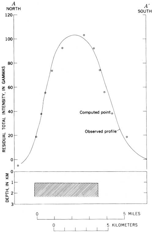
A profile across the Gros Ventre Range (pl. 2, A—A'), from which the regional field has been removed, is shown in figure 11. The computed model is a combination of models A69 and A70 (Vacquier and others, 1951); the standard deviation of the computed points is ±4ϒ. The computed body is oversimplified; but because of the ruggedness of the topography, a more detailed model would be impractical. The apparent volume susceptibility contrast for this model is 0.0004 emu, assuming induced magnetization only. The calculated source is 1.2 km below the flight elevation, or 2.5 km. This elevation is about 300 m below the contact between the Mesozoic and Paleozoic rocks (pl. 1), which indicates that the anomaly source is at the top of the Precambrian rock. (See table 1.) The susceptibility is appropriate for the layered gneisses, assuming negligible susceptibility for the granite and granite gneisses, and it suggests a magnetite content of 0.05-0.10 percent (Lindsley and others, 1966). This amount is consistent with Reed's modal analyses (tables 2-4 of this report).

FIGURE 11.—Observed residual total magnetic intensity profile over Gros Ventre Range anomaly compared with theoretically computed points of model (shaded) shown. Body extends to infinite depth. ΔKa=0.0004 emu, and is the apparent susceptibility contrast. Depth below flight-line elevation is shown. Standard deviation of computed points is ±4ϒ. A—A' is shown on plate 2.

Depth estimates show the source of the Gros Ventre Range anomaly east of the computed profile to be virtually at the bedrock surface, which indicates that the Paleozoic rocks there must be thin. Depth estimates in the Teton Range indicate that the source is at the surface, which implies that the contacts between the magnetic and nonmagnetic rocks are fairly steep.

In the northern Teton Range the magnetic contours associated with the layered gneiss extend over Jackson Lake, which indicates a fairly shallow depth to the layered gneiss and supports the seismic and gravity interpretation of the location of the Teton fault.

The total magnetic intensity map (pl. 2) shows a large anomaly of 400ϒ in the Gros Ventre Range trending off the east edge of the mapped area. This anomaly is not complete enough for a thorough analysis, but it can be associated with a basement feature. At the southern steep gradient, the depth to the crystalline source is estimated to be 300 m.

Precambrian rocks occur at the surface at the extreme edge of the mapped area (pl. 1). A preliminary field check of the area by J. D. Love shows that these rocks are chiefly granite and granite gneiss, and that they surround many bodies of mafic rocks and are cut by others. Local concentrations of magnetite and hematite were observed within this complex. In addition, the Flathead Sandstone (Cambrian) directly overlying the Precambrian rocks has several beds containing moderate amounts of hematite.

The diabase dikes, with one exception, are not shown on the magnetic maps because flight elevations were too high for the effects of these thin bodies to be recorded. The prominent dike on Mount Moran, which was crossed by one flight line only 580 m above the surface, showed a residual anomaly of about 30ϒ. A depth calculation showed that the source is at the surface, as would be expected for a dike. A ground traverse across this dike showed an anomaly of only 700ϒ; so it is not surprising that the effect is negligible on the aeromagnetic profiles.

The residual magnetic map (pl. 3) shows a low (centered near Slide Lake) to the south of the gravity minimum (centered near the east end of Jackson Lake), which would not be expected if the magnetic low were the result of the thickest part of the sedimentary section. This negative anomaly is probably the result of lithologic contrasts within the Precambrian basement. The contrasts, perhaps, are caused by the continuation, east of the Teton fault, of the relatively nonmagnetic granitic rock which is bounded on the north and south by layered gneiss. Depth estimates, based on the observed profiles, were made about 6 km south of seismic line 2. These estimates gave a depth of 4,300 m below the surface, which is slightly shallower than the depth to basement along line 2 (fig. 7) but which is within the error of the method. The origin of this gradient is probably the contact between the granitic rocks and the more magnetic layered gneiss to the north, which continues beneath Jackson Hole east of the Teton fault.

The volcanic rock in the area, with three exceptions, appears to be virtually nonmagnetic, as would be expected because most of this rock is very silicic (Carey, 1956). Two 40ϒ to 60ϒ positive anomalies near the north edge of the area are associated with rhyolite flows (Love, 1956c). A 20ϒ anomaly is associated with andesite porphyry (Scopel, 1956) of East Gros Ventre Butte. No anomaly was mapped over West Gros Ventre Butte, which contains the same rock, because the flight lines did not cross this area.